
GitHub
The code for the herein described process can also be freely downloaded from https://github.com/fzenoni/bcr-map.
Drawing maps with R
In the last few years the R community has done big steps in providing friendly tools to manipulate tables extended by geographical information. The need to display such information in a simple way, coupled with the prescriptions of tidy data summarized by Hadley Wickham (https://www.jstatsoft.org/article/view/v059i10) led to the development of R packages such as sf and tmap, as well as considerable improvement of the well-known R graphic library, ggplot2. Moreover, it is a celebrated fact that data has never been more available than today: thanks to the osmdata package, it is now also easier than ever to extract geographical information from OpenStreetMap (OSM) databases, while staying in the R ecosystem. This package acts as a smart interface between the user and the dreaded official OSM query language, called Overpass.
With this geographical “holy trinity” in the making at our disposal (even though tmap still silently makes conversions from sf to the older sp objects), it is therefore possible for beginner users to set-up fast, but also reproducible workflows. In fact, when dealing with Geographical Information Systems (GIS) a traditional approach consists in opening a GIS program with a GUI, such as QGIS or ArcGIS, and start clicking around one’s way through the building of an appropriate map. The R tools at our disposal, in turn, allow the user to keep full track of his or her actions, maintain this track and share it with other users.
As an exercise, I’m going to display the boundaries of the municipalities located in the Belgian region of Brussels-Capital. Despite the fact that the workflow is rather linear on paper, some caveats and a critical approach are still necessary, and this is what motivated me to write this blog post. My approach to this matter is certainly not original, and I don’t expect to teach anything new to the more experienced R users. On the contrary, real R beginners may struggle in following some of the language shortcuts.
So, let’s start.
Extraction of the political boundaries
To identify our region of interest, we must know a few definitions. As we decided to access the OSM database, we must use whatever key and values are the most used by the community. Administrative boundaries are not internationally defined in a unique way, so we must check how specific countries deal with these different levels. The reference webpage is the following: http://wiki.openstreetmap.org/wiki/Tag:boundary%3Dadministrative. We’re then able to find out that Belgian municipalities are described by level 8.
boundaries <- opq(bbox = 'Brussels, Belgium') %>%
  add_osm_feature(key = 'admin_level', value = '8') %>%
  osmdata_sf %>% unique_osmdata
We can now extract the actual geometrical boundaries from this object…
municipalities <- boundaries$osm_multipolygons… And quickly display it thanks to the tmap::qtm() function.
qtm(municipalities)
Filtering the municipalities
A naive strategy
This seems like a lot of towns, certainly too much for the sole Brussels-Capital Region! Indeed I queried objects inside some rectangular bounding box of the city, defined by Overpass itself. In an ideal world however, we could filter the 19 relevant commune’s names by selecting for instance their postcodes. We know that postcodes inside Brussels Region are included between 1000 and 1210.
# Unfactor addr.postcode column
municipalities <- municipalities %>% mutate(addr.postcode = as.character(addr.postcode))
municipalities <- municipalities %>% mutate(addr.postcode = as.numeric(addr.postcode))
# Filter table
filtered_bxl <- municipalities %>% filter(addr.postcode >= 1000 & addr.postcode <= 1210)
qtm(filtered_bxl)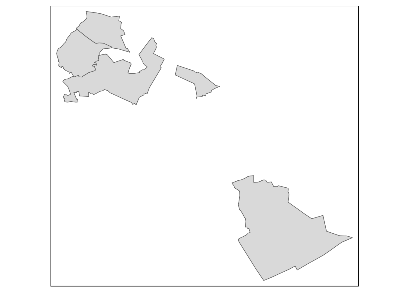
But this is not good either! Indeed, let’s have a look at the original dataset. For the sake of space I’ll only show the first few entries.
table <- municipalities
# Remove geometry from table
st_geometry(table) <- NULL
knitr::kable(head(table[, c('name', 'addr.postcode')]))| name | addr.postcode |
|---|---|
| Saint-Gilles - Sint-Gillis | NA |
| Forest - Vorst | NA |
| Ixelles - Elsene | NA |
| Etterbeek | NA |
| Uccle - Ukkel | NA |
| Anderlecht | NA |
Other boundaries to the rescue
First lesson learnt. We easily notice that, as it often happens when scraping online data, information is incomplete, and many postcodes are missing. Since we do trust the geographical information reported by OSM, we therefore need to think of another strategy, independent of whatever other information OSM databases may or may not include. In the first query we specified the number 8, corresponding for Belgium to the administrative level of Municipalities. As regions are identified by number 4, we can rely on that one to select more precisely our boundaries of interest.
regions <- opq(bbox = 'Brussels, Belgium') %>%
  add_osm_feature(key = 'admin_level', value = '4') %>%
  osmdata_sf %>% unique_osmdata
bxl_region <- regions$osm_multipolygons %>% filter(osm_id == '54094')
qtm(bxl_region)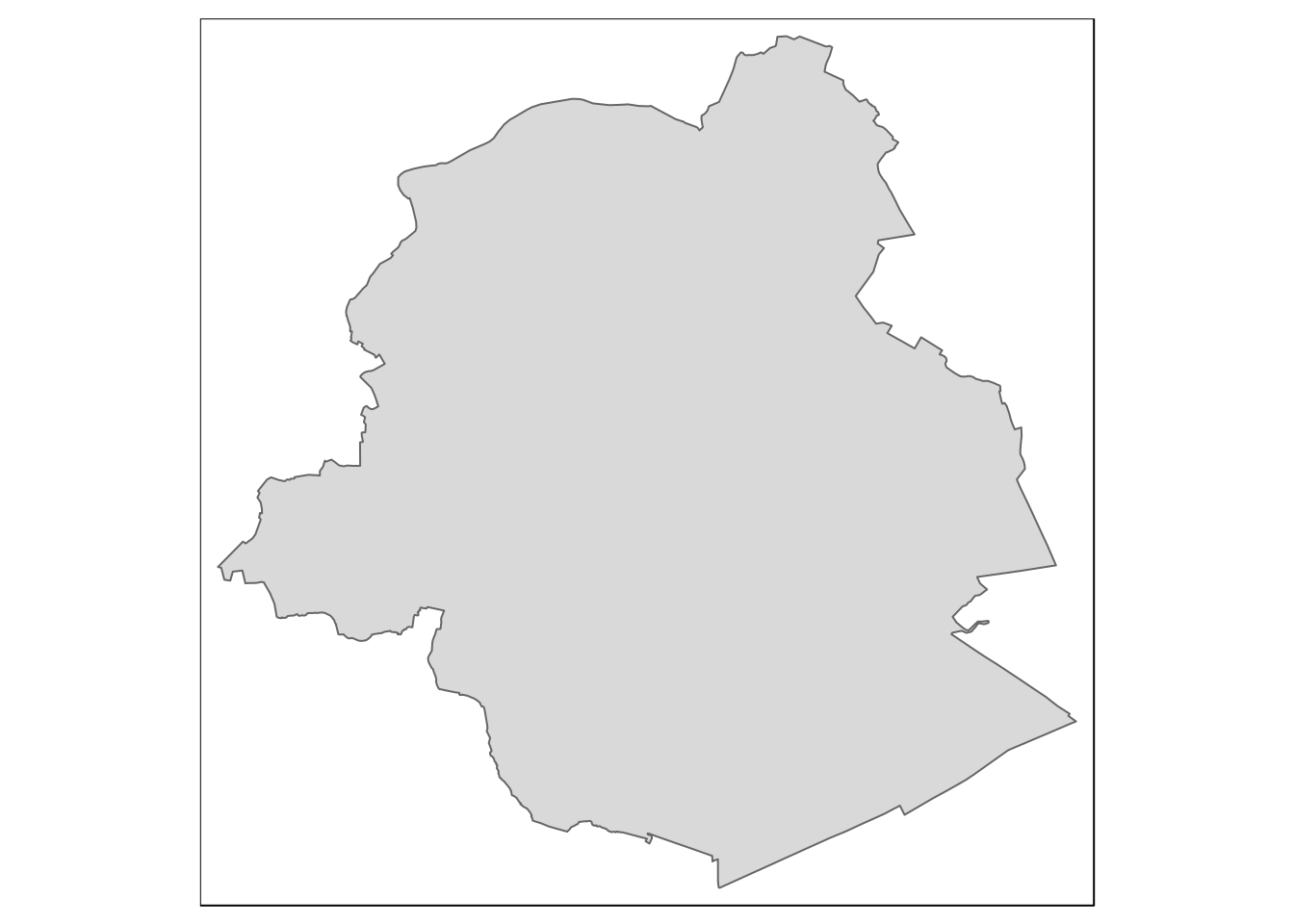
Now we have the shape of Brussels-Capital, but how do extract the municipalities inside of these boundaries? The general, documented way to perform such an operation is trivial.
qtm(municipalities[bxl_region, ]) +
  tm_shape(bxl_region) + tm_borders(col = 'red') # Overlay Brussels region borders in red
Unfortunately, it seems that municipalities immediately outside of the Brussels region (whose borders are highlighted in red for clarity) are still included. This is probably due to the inclusion of the lines common to internal and external municipalities, and the entire polygons that includes them.
Two options
At this point, there may be a few different options. At first, I decided to go through explicit intersection of polygons. However, we need valid polygons in order to do that (and OSM polygons are invalid more often than not). In order to fix broken polygons, you will need to link the sf package against the liblwgeom library installed for your machine. I’ve never managed to install this library on Windows, so leave your solution in the comments if you know how to do it! In any case we’re going to project the map on the appropriate CRS (ETRS89 / Belgian Lambert 2008). The output of the intersection partially consists in line strings, as I suspected from the default subset operation. We don’t need them for the display, so we identify and exclude them. The following works.
municipalities <- st_transform(municipalities, 3812)
bxl_region <- st_transform(bxl_region, 3812)
# Fix the polygons before the intersection, or it will fail
if(!all(st_is_valid(municipalities))) {
  municipalities <- municipalities %>% st_make_valid()
}
bxl_municipalities <- st_intersection(municipalities, bxl_region)
# Select the polygons. The elements with an index greater than 19 are linestrings.
bxl_municipalities_poly <- bxl_municipalities[1:19, ]
Later however, I realized that it was also possible to compute a negative buffer from a polygon, which may represent a more compact, if not “softer”, option in this case, which I adopt.
neg_buffer <- st_buffer(bxl_region, -100) # in meters
bxl_municipalities_poly <- municipalities[neg_buffer, ]
Final act
At this point we can make use of one of the two bxl_municipalities_poly objects that we computed, as they are identical.
# Drop the municipalities factors excluded from the latest subset operations
# or they will appear in the legend.
bxl_municipalities_poly <- bxl_municipalities_poly %>% mutate(name = droplevels(name))
tm_shape(bxl_municipalities_poly) +
  tm_polygons(title = 'Municipalities', col = 'name') +
  tm_layout(legend.outside = TRUE)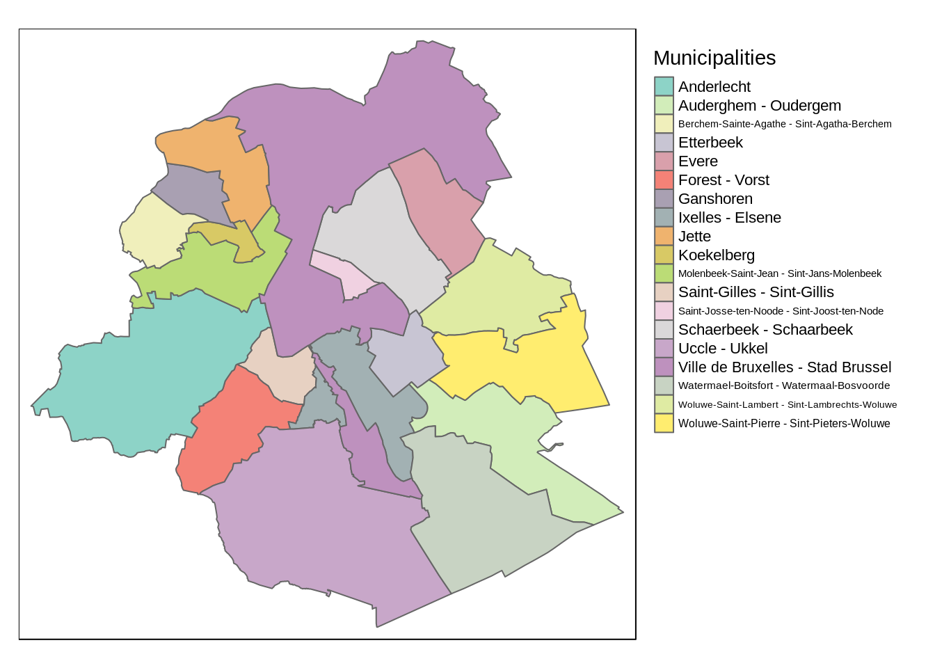
That’s it! We can make the map a little prettier by adding some details. Also, colors could be improved.
tm_style_col_blind() +
  tm_shape(bxl_municipalities_poly) +
  tm_polygons(title = 'Brussels Capital Municipalities', border.col = 'grey40', col = 'name', alpha = 0.6) +
  tm_shape(bxl_region) + tm_borders(col = 'grey20', lwd = 2, alpha = 0.8) +
  tm_layout(legend.outside = TRUE, frame.double.line = TRUE) +
  tm_grid(projection = 'longlat', n.x = 5) + tm_scale_bar() +
  tm_compass(position = c('right', 'top'))
I’m still not completely satisfied, but with more time and some more experience in data visualization things could be improved. Anyway, it’s a good start.
On the next episode we’ll see how to deal with a port city: how can we display the coastline?
Acknowledgements
I would like to thank Timo Grossenbacher (https://timogrossenbacher.ch) for the public release of his “template for bootstrapping reproducible RMarkdown documents for data journalistic purposes”. You may clone it from here: https://github.com/grssnbchr/rddj-template.