
GitHub
The code for the herein described process can also be freely downloaded from https://github.com/fzenoni/coast-map.
Where were we
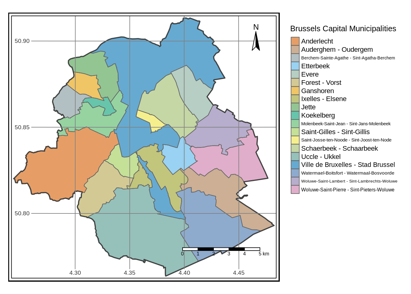
In the previous post (click here if you missed it), we managed to put together a relatively short chunk of code that generated the following rather nice map of Brussels Region, which includes all of its 19 municipalities.
A new challenger appears
In that post, we discussed how a certain amount of challenges were overcome. We picked Brussels, a city that lays in mainland. As a consequence, we did not have to worry about what stands around Brussels, because it wouldn’t have added much information to our map. But what if instead we decided to display a city on the coast? For this purpose, let’s choose a warmer place, such as Bilbao, Spain! Besides the presence of the sea, this choice will give us the chance check how to visualize Bilbao’s estuary, and also possibly the flowing river. The main challenge is to do all of this without relying on any manually downloaded data: everything will come directly from OSM databases, osmdata package being the intermediary.
You’ll get there, quick, Red Riding Hood, if you take the shortcut, through the woods
Packages such as cartography, despite proposing a quick way to access the shapes of the world’s countries, severely lack in resolution when a single city needs to be visualized. A valid, alternative approach to the method presented from here on would be to download the complete coastlines of Earth. They’re available in the Shapefile format at the following link.
At this stage I should also specify that tmap gives you the chance to superimpose your queries to the OpenStreetMap map tiles, by creating an interactive HTML widget. This could be the shortest possible answer to display the region of interest in its geographical context. To showcase this let’s begin once again by the fundamentals. We are going to query the administrative level 7, corresponding the the comarca of Greater Bilbao (some sort of Spanish equivalent of the county administrative division).
boundaries <- opq(bbox = 'Bilbao, Spain') %>%
  add_osm_feature(key = 'admin_level', value = '7') %>%
  osmdata_sf %>% unique_osmdata
Now let’s activate the “view” option (the default being “plot”), and let’s display the region we queried.
tmap_mode('view')
qtm(boundaries$osm_multipolygons[5,])
It’s a cool solution when building websites or interactive presentations. But it’s not optimal when a map needs to be printed and the programmer wants to highlight specific aspects of the map.
# Reset to default for next steps
tmap_mode('plot')
## tmap mode set to plottingYou know it ain’t easy, You know how hard it can be
We know how to query boundaries with osmdata; nothing stops us from querying a coastline. But first, I will define a slightly larger bounding box, so that we are mathematically sure that our boundaries, as well as their land and see surroundings will be correctly displayed in the final picture.
bb <- st_bbox(boundaries$osm_multipolygons[5,])
# Defining a buffer
buffer <- 0.1
p_big <- rbind(c(bb[1] - buffer, bb[2] - buffer),
  c(bb[1] - buffer, bb[4] + buffer),
  c(bb[3] + buffer, bb[4] + buffer),
  c(bb[3] + buffer, bb[2] - buffer),
  c(bb[1] - buffer, bb[2] - buffer))
# Putting the coordinates into a squared polygon object
pol <- st_polygon(list(p_big)) %>% st_geometry
# Providing the SRID (here, unprojected lon/lat)
st_crs(pol) <- 4326
The correct key and value to obtain the coastline are natural and coastline (check the wiki page for more details).
coast <- opq(bbox = st_bbox(pol)) %>%
  add_osm_feature(key = 'natural', value = 'coastline') %>%
  osmdata_sf %>% unique_osmdata

qtm(coast$osm_lines)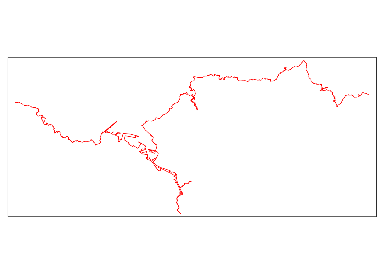
Interesting already! We got Bilbao’s coastline as well as the estuary. We can quickly superimpose what we have.
qtm(boundaries$osm_multipolygons[5,]) + qtm(coast$osm_lines)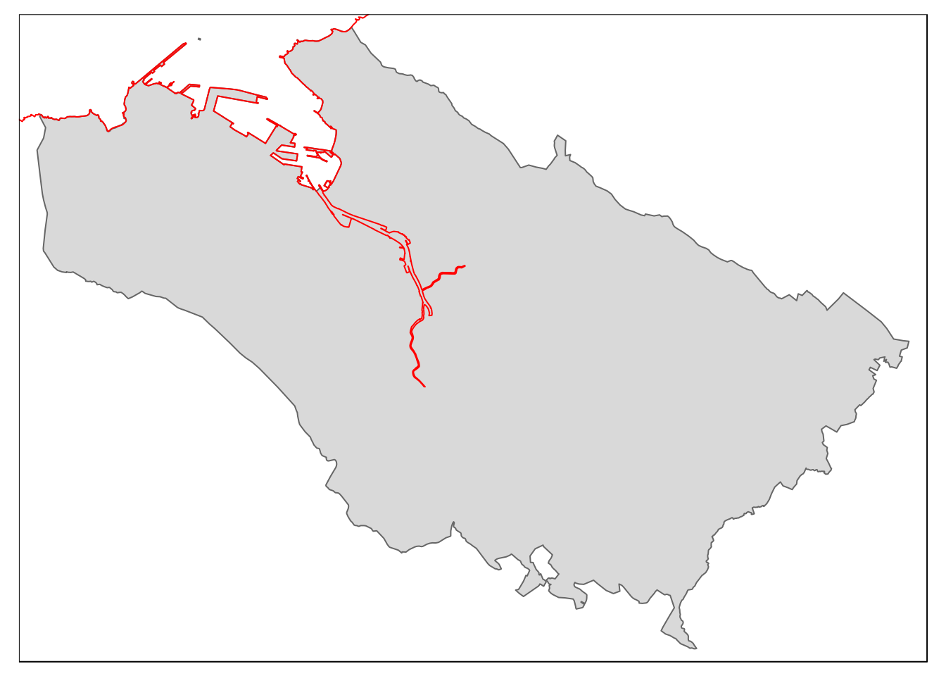
Is there more to it? Can we see the rest of the river? To find out, I am going to query any OSM object carrying the key waterway.
water <- opq(bbox = st_bbox(pol)) %>%
  add_osm_feature(key = 'waterway') %>%
  osmdata_sf %>% unique_osmdata
After a quick inspection, it seems that the watercourses are represented as polygons. Let’s add them to the rest.
qtm(boundaries$osm_multipolygons[5,]) + qtm(coast$osm_lines) + qtm(water$osm_polygons)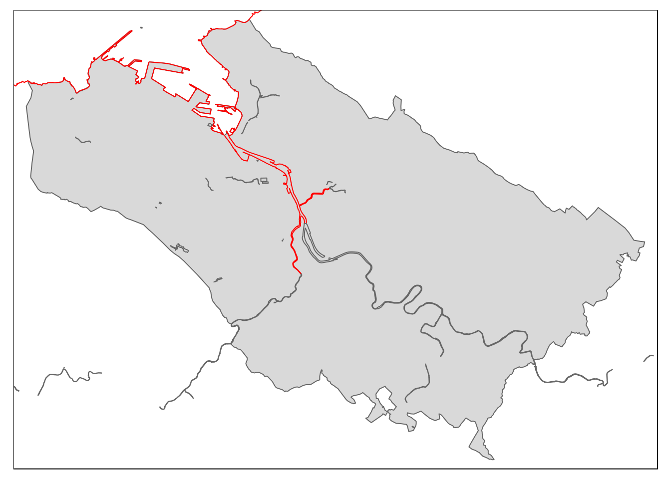
It is a very rough visualization, but as one can guess, almost all the elements are here.
Now, no map of a coastal city would be complete without appropriate colors for sea and land. If land and sea were uniquely represented by polygons, this would be an easy task. Instead, all we have, at least for the coastline, is a data.frame of LINESTRING objects. The strategy would then be to cut the polygon frame in two parts, according to the coast acting as a “blade”. Luckily for us, the sf package includes many of the functions available in PostGIS technology. This time, it’s the time for st_split() to shine. You will need to install the liblwgeom library to use it: check this Github repository for more information.
N.B.: Things did not exactly go as expected for this blog post. I still pay the price for some lack of experience. In the following lines, if you know a better solution, or understand what is going wrong, don’t hesitate to write in the comments!
First, we define the blade by taking the coastline, making a union of all the data.frame rows, thus obtaining a MULTILINESTRING. After inspection, that object is truly a single string, so we use the appropriate function to merge everything. This is very important, because st_split() does not support cutting a polygon with a multilinestring (as reported in the PostGIS doc).
blade <- coast$osm_lines %>% st_union %>% st_line_mergeWe use this blade to cut the squared polygon we defined earlier.
multipol <- st_split(st_geometry(pol), st_geometry(blade))The result is a GEOMETRYCOLLECTION. In principle, one could access the different elements of the collection (in this case, two) by using double square brackets. For a reason I could not understand, in this case it works only for the first element, which I then cast appropriately.
land <- st_cast(multipol[[1]], 'POLYGON') %>% st_geometry %>% st_sf
st_crs(land) <- 4326
This is why, instead of calling the second polygon with multipol[[2]], I am forced to make a different kind of operation. Looking at the bright side, this is yet another display of possible sf geometrical operations.
sea <- st_difference(pol, land) %>% st_geometry %>% st_sf
st_crs(sea) <- 4326
We are now ready to display everything, similarly to what was done in the last post. Note the is.master = T activated option, which calibrates the borders of the final picture according to Bilbao’s boundaries, instead of the polygon called first (in this case, land).
tm_shape(land) + tm_polygons(col = 'bisque3', alpha = 0.8) +
  tm_shape(boundaries$osm_multipolygons[5,], is.master = T) + tm_polygons() +
  tm_shape(sea) + tm_polygons(col = 'skyblue', alpha = 0.8) +
  tm_shape(water$osm_polygons) + tm_polygons(col = 'skyblue', alpha = 0.8) +
  tm_grid(n.x = 5, projection = "longlat") +
  tm_layout(legend.outside = TRUE, title = 'Bilbao, Spain', frame.double.line = TRUE) +
  tm_scale_bar() + tm_compass(position = c('right', 'top'))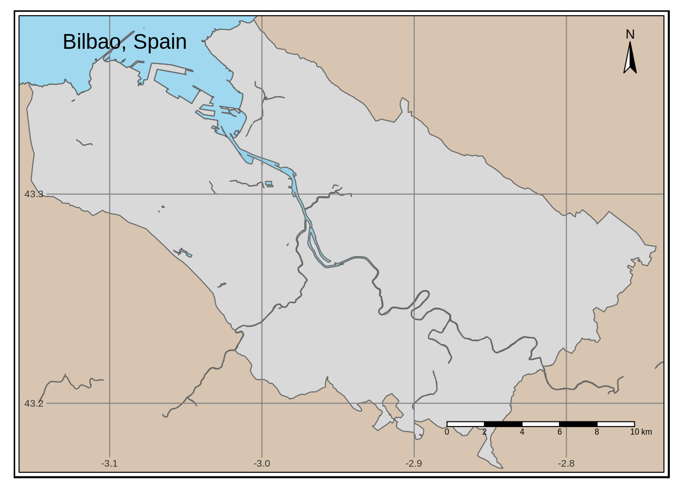
Conclusions
In this post I’ve just shown how to rely exclusively on the GIS R package trinity sf, osmdata, and tmap, to build a display the boundaries of an administrative city together with some more geographical information. Unfortunately, it is difficult to automate this procedure, essentially because of the st_split() operation and the appropriate definition of a blade. In fact, depending on the geographical region, the query for coastlines could return islands. It is then up to the user to put together the specific segments that form a single line, able to divide the bounding box in two parts.
To deal with islands, also delimited by LINESTRINGS, and treat them as polygons, one suggestion would be to apply the st_polygonize() function to these closed lines, to eventually overlay them in the usual tmap way. The needed dedication, and the time consuming aspects of this series of tasks are probably representative of the somewhat fading distinction between art and data science.